Choosing a modeling approach

Optimality models are useful when we focus on a single individual in a contest against "NATURE" (all environmental variable lumped together)

Such an approach works if none of the components that make up "NATURE" respond to an animal's strategy (i.e. they don't change their behavior or relationship towards the focal animal and its behavior)

If "NATURE" responds, theorists often turn to Game Theory

 

Computing payoffs:

Strategies almost universally affect several components of fitness simultaneously, usually in opposite ways (because they involve investments of time and energy toward one thing..... this takes away from another).

 

Calculating payoffs involves the combination of various costs and benefits:

 

We will consider two types of payoffs: Simple and Conditional

 

Simple payoffs result from completely predictable benefits (B) and costs (C).

Animals will often try to maximize some relationship between B and C (e.g., B - C or B/C).

 

Conditional payoffs result when B & C are fixed, but the probability of experiencing the benefit or cost is less than 1. There are many possibilities

 

1) For example, a strategy will lead to a benefit (B) with probability p. If an animal doesn't get B, it gets some cost (-C) at probability (1 - p).

The expected payoff is: p(B) +(1-p)(-C)

 

2) Another example: an animal does a behavior at cost -C that produces a benefit (B) with probability p (and no benefit with probability 1-p). In either case, the animal accepts the cost (-C)

Now the average expected payoff is: p(B-C) + (1-p)(-C) = pB - C

 

Remember, the sum of all probabilities must equal 1, this helps if there are more that one type of benefit or cost.

Click here for a couple practice questions that involve Optimality Theory

Optimality models typically assume:

Haploid or clonal reproduction (sex complicates estimates of fitness, but may not alter predictions)

Infinite population size and no subdivision of the population

Strategy set is complete and distinct (i.e., strategies are not subsets of other strategies that are included in the same model)

The optimal solution is genetically possible (e.g., flying elephants!)

 

Using optimality to understand the economics of prey choice or foraging behavior

 

First, an example of a discrete optimality model: Choice of two prey with different values (see box 3.2, pg 61 in the text)

 

Prey type 1 (P₁) is worth E₁ of energy but takes H₁ to break open

Prey type 2 (P₂) is worth E₂ of energy and takes H₂ to break open

 

P₁ is more valuable than P₂ i.e., E₁/H₁ > E₂/H₂

Obviously, eat every P₁ encountered

 

The decision to skip or eat P₂ will depend on the availability of P₁ (which will influence how long it takes to find the next P₁ measured as the search time (S₁)

 

A forager should eat P₂ when the value of eating P₂ is greater that the value of P₁, discounted by the time needed to search for the next one: [i.e. E₂/H₂ > E₁/(S₁ + H₁)]. This leads to the inequality: S₁ > (E₁H₂/E₂) - H₁

 

Three predictions emerge from this result:

a) Predator should either: just eat P₁ (specialize); or eat both P₁ and P₂ (generalize)

b) Switch should depend only on S₁ (availability of P₁ ) not the density of P₂ (S₂)

c) The switch from specialized to generalized feeding should be abrupt

 

An example of a continuous optimality model: Marginal value analysis of optimal feeding time in food patches (see box 3.1, pg 56 for another application of the marginal value theorum)

Marginal value ideas focus on diminishing returns and the timing of giving up or abandoning a strategy of resource exploitation

1) Assume prey are dispersed in "patches" (some areas better than others)

2) Assume the value of patches declines with time (e.g., depletion)

3) Assume patches are initially of equal value

4) Assume patches are distributed evenly (equal travel time between patches)

 

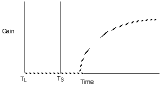
Diminishing return models for single prey types generate decelerating curves through time (measured as cumulative gain or proportion of total gain)

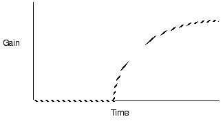
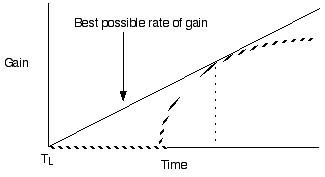
Violate assumption 3: Varying patch quality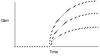

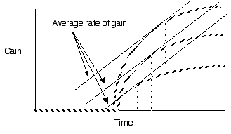
Predict longer residency in the better patches

Violate assumption 4: Varying travel time between patches

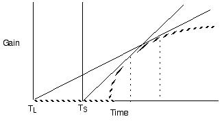
Predict shorter residency when patches are closer together

Other tacit assumptions: perfect knowledge of patch value and distribution... this may explain why animals sometimes stay longer than predicted in bad patches.