The quest of Behavioral Ecology: why do animals behave as they do?

To understand behavioral ecology, we must understand the link between the expression of behaviors and individual fitness.

Remember the big three: Food, Sex, and Death

 

Diversity in behavior can be examined as a function of animal Social Organization (where animals are found and who interacts with whom)

Primary Social Organization: Behaviors that relate directly to temporal and spatial patterns of distribution (grouping, spreading out, etc.)

 

Higher-order Social Organization: Behaviors that relate to social interactions among animals (mating systems, parental care, cooperation, etc.)

 

Why treat dispersion separately from social behavior issues? After all, most patterns of dispersion involve some level of social interaction?

Patterns of dispersion (the frequency and consistency of encounters between individuals) establish the "template" for social interactions.... selection for "higher order" social behaviors.

 

Why is math important to the study of animal behavior?

Mathematical methods demand explicit formulations (in contrast to the vagueness of many verbal arguments

 

Models are useful for developing general concepts that may apply to many different types of organism

 

Models may suggest non-intuitive relationships

 

Caveats:

Models often rely on overly simple assumptions,

Testing models can be problematic (are the data lacking or is the model wrong?)

Hypotheses generated by models may be neither exclusive, nor exhaustive

 

Still, mathematical treatments of animal behavior can be very useful IF you understand the method behind the madness

Three basic sources of theory in behavioral ecology:

Comparative methods

Optimality theory

Game theory

Comparative methods can be useful for identifying generally important aspects of behavior, but theory is often post hoc.

Overview of quantitative theoretical approaches to the study of animal behavior

Both optimality and game theory seek to answer the same question: given a particular ecological scenario (physical and social environmental conditions) for a given individual, should it continue a set of behaviors or adopt some alternative?

Definitions:

Strategies: the options available to an animal (no decision making implied!)

Alternative strategies can either be discrete or continuous.

 

Payoffs: the net effect on fitness associated with a specific strategy (assumes strategies have both costs and benefits)

 

Many variables may influence fitness, though only a subset may be relevant to the model.

 

Thus, choice of a "currency" that relates to fitness is important

 

Overall Lifetime Inclusive Fitness (OLIF) is the only complete currency

It is virtually impossible to measure

 

Proxies for OLIF usually relate to one of the big three (food, sex, or death)

 

Choosing a modeling approach

Optimality models are useful when we focus on a single individual in a contest against NATURE (all environmental variable lumped together)

Such an approach works if none of the components that make up NATURE respond to an animal's strategy (i.e. they don't change their behavior or relationship towards the focal animal and its behavior)

If NATURE responds, theorists often turn to Game Theory

 

Computing payoffs:

Strategies almost universally affect several components of fitness simultaneously, usually in opposite ways (because they involve investments of time and energy toward one thing..... this takes away from another).

 

Calculating payoffs involves the combination of various costs and benefits:

 

We will consider two types of payoffs: Simple and Conditional

 

Simple payoffs result from completely predictable benefits (B) and costs (C).

Animals will often try to maximize some relationship between B and C (e.g., B - C or B/C).

 

Conditional payoffs result when B & C are fixed, but the probability of experiencing the benefit or cost is less than 1. There are many possibilities

 

1) For example, a strategy will lead to a benefit (B) with probability p. If an animal doesn't get B, it gets some cost (-C) at probability (1 - p).

The expected payoff is: p(B) +(1-p)(-C)

 

2) Another example: an animal does a behavior at cost -C that produces a benefit (B) with probability p (and no benefit with probability 1-p). In either case, the animal accepts the cost (-C)

Now the average expected payoff is: p(B-C) + (1-p)(-C) = pB - C

 

Remember, the sum of all probabilities must equal 1, this helps if there are more that one type of benefit or cost.

 

Optimality models typically assume:

 

Haploid or clonal reproduction (sex complicates estimates of fitness, but may not alter predictions)

Infinite population size and no subdivision of the population

Strategy set is complete and distinct (i.e., strategies are not subsets of other strategies that are included in the same model)

The optimal solution is genetically possible (e.g., if pigs could fly......)

 

An example of a discrete optimality model: Choice of two prey with different values

 

Prey type 1 (T₁) is worth E₁ of energy but takes H₁ to break open

Prey type 2 (T₂) is worth E₂ of energy and takes H₂ to break open

 

T₁ is more valuable than T₂ i.e., E₁/H₁ > E₂/H₂

Obviously, eat every T₁ encountered

 

The decision to skip or eat T₂ will depend on the availability of T₁ (which will influence how long it takes to find the next T₁ measured as the search time (S₁)

 

A forager should eat T₂ when the value of eating T₂ is greater that the value of T₁, discounted by the time needed to search for the next one: [i.e. E₂/H₂ > E₁/(S₁ + H₁)]. This leads to the inequality: S₁ > (E₁H₂/E₂) - H₁

 

Three predictions emerge from this result:

a) Predator should either: just eat T₁ (specialize); or eat both T₁ and T₂ (generalize)

b) Switch should depend only on S₁ (availability of T₁ ) not the density of T₂ (S₂)

c) The switch from specialized to generalized feeding should be abrupt

 

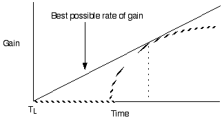
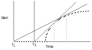
An example of a continuous optimality model: Marginal value analysis of optimal feeding time in food patches:

1) Assume prey are dispersed in "patches" (some areas better than others)

2) Assume the value of patches declines with time (e.g., depletion)

3) Assume patches are initially of equal value

4) Assume patches are distributed evenly (equal travel time between patches)

 

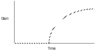
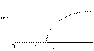
Diminishing return models for single prey types generate decelerating curves through time

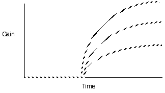
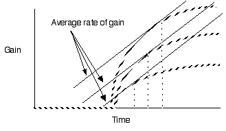
Violate assumption 3: Varying patch quality

Predict longer residency in the better patches

Violate assumption 4: Varying travel time between patches

Predict shorter residency when patches are closer together

Other tacit assumptions: perfect knowledge of patch value and distribution... this may explain why animals sometimes stay longer than predicted in bad patches.